Applying crystal data
| 2D simulation of reciprocal space | Structure factors |
| Atomic scattering factors | Unit cell transformation |
Another tutorial covers the import of crystal data to the format used in this package. In this tutorial we will see a few examples on how to make use of that information.
| In[1]:= |
This package comes with many convenient functions that utilises the stored crystal data. They can mainly be divided into two categories: those used to extract data and those used for calculations.
| GetAtomicScatteringFactors† | returns |
| GetCrystalMetric | return the metric |
| GetLatticeParameters | return the lattice parameters associated with the crystal |
| GetLaueClass | returns the corresponding Laue class of the group/crystal |
| GetScatteringCrossSection† | returns σ for given elements and wavelength |
| GetSymmetryData | extract space group information easily |
| GetSymmetryOperations | returns alle the symmetry operations for a point- or space group |
| ImportCrystalData | import crystallographic information from cif files |
Functions that are mainly used for easy extraction of data.
† denotes functions that use data files located $MaXrdPath ▶ Core ▶ Data.
| AttenuationCoefficient | calulate the μ abosrption factor |
| BraggAngle | calculate the Bragg angle, given λ and hkl |
| CrystalDensity | calculate theoretical value for the density |
| DarwinWidth‡ | calculate the Darwin width of a given hkl |
| ExtinctionLength‡ | calculate the extinction (Pendellösung) distance of a given hkl |
| ReciprocalSpaceSimulation | simulate the reflections (nodes) of a plane in reciprocal space |
| StructureFactor | calculate the structure factor |
| UnitCellTransformation | transform among alternative unit cell representations |
Functions in the package which can operate on data in $CrystalData, $PointGroups or $SpaceGroups directly to perform calculations.
‡ denotes functions related to dynamical diffraction theory.
2D simulation of reciprocal space
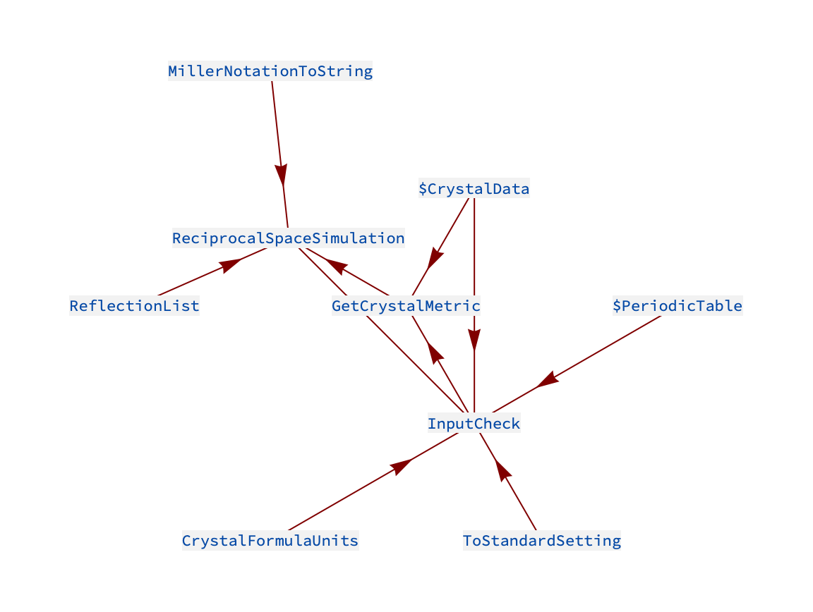
With the metric information of a crystal contained in $CrystalData and the function for generating appropriate reflections, ReflectionList, one can relatively easily create a function that simulates a section of reciprocal space. ReciprocalSpaceSimulation is a simple function that does this. We can use RelatedFunctionsGraph to check which other package components it is made of:
The essential inputs are the crystal label – which contains the lattice specification – and the orientation details of the plane in reciprocal space. Information on the function syntax:
From this we see that the function also requires an origin for the plane, a resolution and wavelength (if not contained along with crystal data). Let us look at some examples:
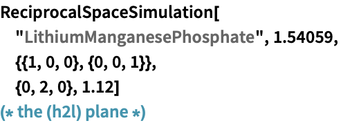
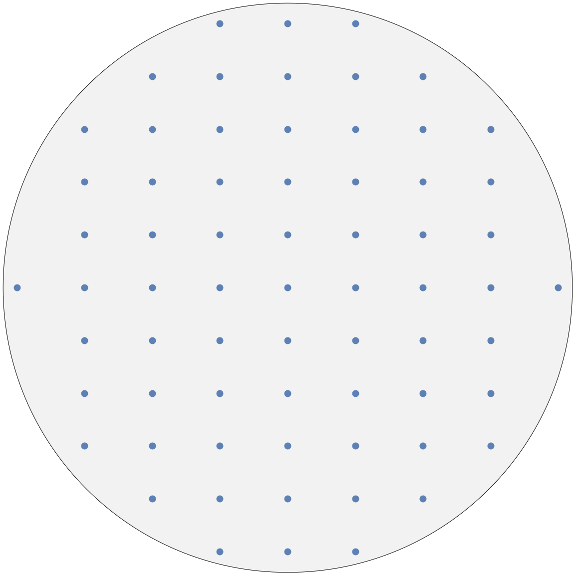
The image above shows the ![]() plane of an orthorhombic structure.
plane of an orthorhombic structure.
Below is an example of a hexagonal structure:
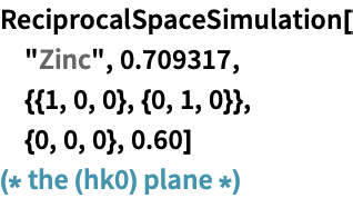
Adjusting the resolution will have the effect of “zooming” in and out. The resolution governs which reflections we are able to see. Note that the indices of the reflections can be read from the tooltips (hover the mouse over any node).
Please see the documentation page for more example of usage.
Atomic scattering factors
The GetAtomicScatteringFactors function return ![]() from either crystal and reflection input or element and
from either crystal and reflection input or element and ![]() input. This function requires sources of coefficients or interpolation functions in order to produce the results, and since the documentation page contains example on use, this tutorial will elaborate on the origin of the source tables included in this package.
input. This function requires sources of coefficients or interpolation functions in order to produce the results, and since the documentation page contains example on use, this tutorial will elaborate on the origin of the source tables included in this package.
Sixteen .dat files are available at ESRF's FTP server, with prefix f0 for files regarding the ![]() factor and prefix f1f2 for the
factor and prefix f1f2 for the ![]() factors. After retrieving these (late 2017) they were prepared in a format to be imported by Mathematica when needed.
factors. After retrieving these (late 2017) they were prepared in a format to be imported by Mathematica when needed.
The data is stored in two different ways: either as coefficients (so-called Cromer–Mann coefficients) to approximate the scattering factor with the function
where ![]() runs from
runs from ![]() to
to ![]() or
or ![]() , or as data points:
, or as data points: ![]() in the f0 cases and
in the f0 cases and ![]() in the f1f2 cases, where
in the f1f2 cases, where ![]() is defined above and
is defined above and ![]() denotes energy. Actually, some files contain more columns, but these are ignored. Energy units are converted to ångströms.
denotes energy. Actually, some files contain more columns, but these are ignored. Energy units are converted to ångströms.
The coefficients method is only available for the f0 case, but some files use the data point method. An overview is given here (third column show valid range; missing means ![]() [truncated]):
[truncated]):
In all cases where data points are used, the Mathematica function Interpolation was used to generate interpolation functions; one for every data pair within each chemical element. Finally, all the interpolation functions were stored as an association with element symbols as keys. This was saved to an m file with the same name as the dat file.
| In[2]:= |
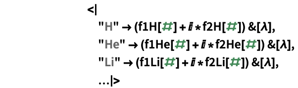
where the f* functions are the corresponding interpolation functions generated, which require a wavelength input and return the value of f0, f1 or f2.
The f0 interpolation functions use interpolation order 3, while the f1f2 functions use order 1 (linear). All use the Hermite interpolation method.
Note that for all f0, f1 and f2 interpolation functions the desired scattering factor is obtained with:
| In[3]:= |
where sourceName denotes one of the associations constructed from any of the dat files storing the information as data points, "element" should be the symbol of a chemical element and the wavelength is in ångströms. A demonstration of this is in order: After using GetAtomicScatteringFactors the first time in a session, the following “hidden” symbols are created:
These associate the file names with the corresponding imported associations.
After running the code above, the symbols are created. Let us check this:
We recognise the default f0 and f1f2 sources. The "WaasmaierKirfel" source contain coefficients:
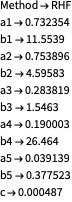
while the "CromerLiberman" source uses data points (as all f1f2 data files):
Structure factors
The StructureFactor function is written in a way that requires minimal input from the user. Syntax information:
Note that the crystal name/label is required and a list of one or more reflections. The wavelength is necessary if not already contained in along with the crystal in $CrystalData.
StructureFactor incorporates several other functions in the package, see the graph below.
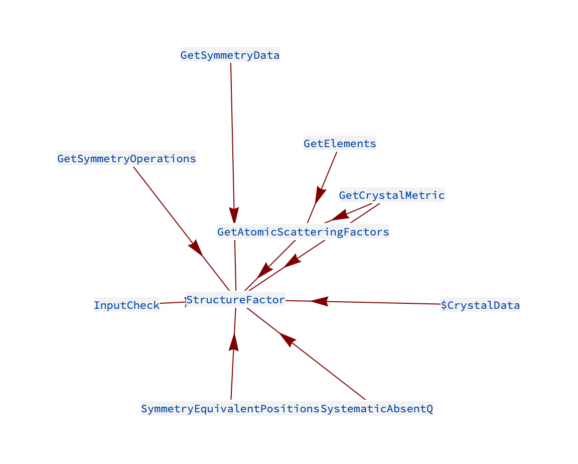
There are also some options available:
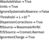
Details are found on the documentation page. Note the options for specifying which sources to use for obtaining the atomic scattering factor (![]() ). The available sources are located in:
). The available sources are located in:
$UserBaseDirectory ▶ Applications ▶ MaXrd ▶ Core ▶ Data ▶ AtomicScatteringFactor
Which in the current version include:

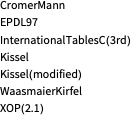
The sources for the anomalous corrections are contained in a subfolder:
$UserBaseDirectory ▶ Applications ▶ MaXrd ▶ Core ▶ Data ▶ AtomicScatteringFactor ▶ AnomalousCorrections

Here are some quick demonstartions for the crystals gallium arsenide and germanium (the wavelength corresponds to ![]() radiation):
radiation):
By default, the modulus and phase are outputted in pairs: ![]() . Complex numbers can be used instead:
. Complex numbers can be used instead:

Please see the documentation page for more example of usage and elaboration on the options.
Unit cell transformation
This package includes the function UnitCellTransformation that transforms entries in $CrystalData among alternative settings of the same space group. In this example we will look at how the metric is transformed, and will be demonstrating this on the crystal ferrocene.

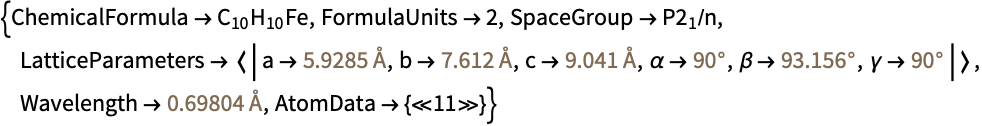
There may be several attributes, such as cell origin, cell choice, axis permutation, centring and so forth. In this case, there are only two setting parameters to fiddle with. We see that the ![]() -axis is the unique axis, which is the standard choice, but the cell choice is set to
-axis is the unique axis, which is the standard choice, but the cell choice is set to ![]() instead of
instead of ![]() .
.
Let us transform the cell so that the ![]() -axis becomes the uniqe axis (the axis with a corresponding angle different from
-axis becomes the uniqe axis (the axis with a corresponding angle different from ![]() ). We can either use the International Tables for Crystallography, volume A or $TransformationMatrices:
). We can either use the International Tables for Crystallography, volume A or $TransformationMatrices:
| In[8]:= |
If we wanted to change the cell choice at the same time, we would simply multiply the two transformation matrices together to a form another matrix ![]() to be used in
to be used in ![]() .
.
We conclude this example with a demonstration of UnitCellTransformation that performs the same transformation of ferrocene as we did «manually»:
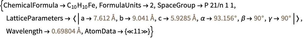
You may notice how the new space group symbol is ![]() . If the symbol is ambiguous, full Hermann–Mauguin symbols are used for non-standard settings.
. If the symbol is ambiguous, full Hermann–Mauguin symbols are used for non-standard settings.
The function UnitCellTransformation also transforms the fractional coordinates and the ADPs (atomic displacement parameters).